In [14]:
import numpy
import matplotlib.pyplot as plt
%matplotlib inline
Frequency response
In [15]:
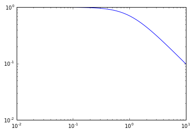
def G(s):
    return 1/(s + 1)
In [16]:
omega = numpy.logspace(-2, 1)
In [17]:
s = 1j*omega
In [18]:
plt.loglog(omega, numpy.abs(G(s)))
Out[18]:
[<matplotlib.lines.Line2D at 0x10e63a390>]
In [19]:
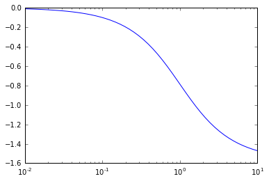
plt.semilogx(omega, numpy.angle(G(s)))
Out[19]:
[<matplotlib.lines.Line2D at 0x10f553f60>]
In [20]:
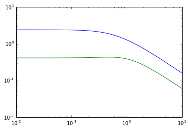
def G(s):
    return numpy.matrix([[1/(s + 1), 0],
                         [2/(2*s + 1), 1/(s + 1)]])
In [21]:
G(s[3])
Out[21]:
matrix([[ 0.99976706-0.01526062j,  0.00000000+0.j        ],
        [ 1.99813777-0.06099987j,  0.99976706-0.01526062j]])
In [22]:
r = []
for si in s:
    r.append(G(si))
In [23]:
r = [G(si)[0,0] for si in s]
In [24]:
r = map(G, s)
In [25]:
sigmas = numpy.array([numpy.linalg.svd(G(si))[1] for si in s])
In [26]:
plt.loglog(omega, sigmas)
Out[26]:
[<matplotlib.lines.Line2D at 0x10f58e860>,
 <matplotlib.lines.Line2D at 0x10ef69f60>]
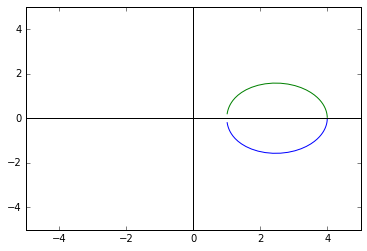
Multivariable Nyquist
In [27]:
I = numpy.eye(2)
dets = [numpy.linalg.det(I + G(si)) for si in s]
In [28]:
plt.plot(numpy.real(dets), numpy.imag(dets))
plt.plot(numpy.real(dets), -numpy.imag(dets))
plt.axis([-5, 5, -5, 5])
plt.axvline(0, color='black')
plt.axhline(0, color='black')
Out[28]:
<matplotlib.lines.Line2D at 0x10f8b16d8>
\[l = \sqrt{a^2 + b^2}\]